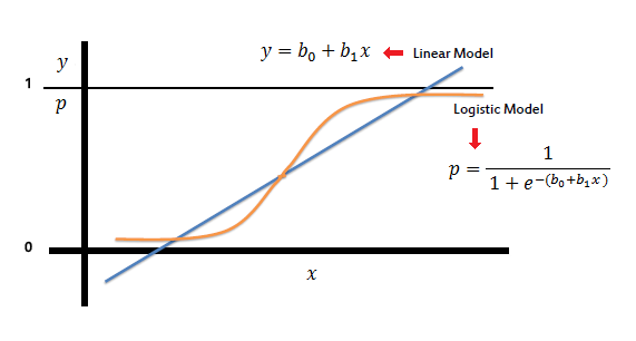
Chapter 4. Classification

• What is classification?

  predicting a qualitative reponse

4.1 An Overview of Classification

**Dataset Introduction **

• default($Y$) : Yes / No
• balance($X_1$)
• income($X_2$)

4.2 Why Not Linear Regression?

• The gap between levels are not exactly same

  ​

  **Then, binary variable? **(dummy variable)

• Estimates can be outside the [0,1] interval

4.3 Logistic Regression

• Logistic regression model predicts the probability that Y belongs to a particular category, rather than the reponse Y directly

  ex.

  

4.3.1 The Logistic Model

• how to set output values between [0,1]?

  logistic function

  ​

  $ p(X) = \frac{e^{\beta_0 + \beta_1X}}{1+e^{\beta_0 + \beta_1X} }$ (4.2)

  

  • S - shaped curve

    ​

    

  • p(X) / [1-p(X)] is called odds, between 0(very low possibility) and infinite(very high possibility)

    

  • log(p(X) / [1-p(X)]) is called the log-odds or logit.

  • $\beta_1$ does not correspond to the change in p(X) associated with a one-unit increase in X

  • The amount that p(X) changed due to one-unit change in X will depend on the current value of X

  • **INCREASING X BY ONE UNIT CHANGES MULTIPLIES THE ODDS BY $e^{\beta_1}$ **

  • $\beta_1$ positive : increasing X -> increase p(X)

    ​

    ​

    ​

  ​

4.3.2 Estimating the Regression Coefficients

• not least squares method

• maximum likelihood

  

  estimates $\hat{\beta}_0, \hat{\beta}_1$ are chosen to maximize this likelihood function(non-linear)

  cf. least square method also a special case of maximum likelihood

4.3.3 Making Predictions

4.3.4 Multiple Logistic Regression

example. How coefficient would be different(positive/negative) between LR and multiple LR?

LR : default & student(Yes) : (+)

multiple LR : default & student(Yes) : (-)

Reason : for a fixed value of balance and income, a student is less likely to default than a non-student -> multiple LR : negative

but, overall student default rate > non-student default rate -> LR : positive

Conclusion : a student is riskier than a non-student if no info about the student’s credit card balance, however, that student is less risky than a non-student with the same credit card balance

*correlation among predictors -> difference between LR & multiple LR called as **confounding** phenomenon*

4.3.5 Logistic Regression for >2 Response Classes

class 3 prob = 1 - class1prob - class2 prob

but in this case -> Linear Discriminant Analysis

4.4 Linear Disciminant Analysis

• What’s the difference between LDA and logistic regression?

Logistic regression involves directly modeling Pr(Y = k|X = x) using the logistic function, for LDA, we model the distribution of the predictors X separately in each of the response classes (i.e. given Y ), and then use Bayes’ theorem to flip these around into estimates for Pr(Y = k|X = x). When these distributions are assumed to be normal, it turns out that the model is very similar in form to logistic regression.

• When LDA?
  • When the classes are well-separated, the parameter estimates for the logistic regression model are surprisingly unstable. Linear discriminant analysis does not suffer from this problem.
  • If n is small and the distribution of the predictors X is approximately normal in each of the classes, the linear discriminant model is again more stable than the logistic regression model.
  • when we have more than two response classes.

4.4.1 Using Bayes’ Theorem for Classification

• $\pi_k$ : the overall or prior probability that a randomly chosen observation comes from the kth class

  = the probability that a given observation is associated with the kth category of the response variable Y

• $f_k(X)$ ≡ Pr(X = x

  Y = k) : the density function of X for an observation that comes from the kth class.

  • if large, there is a high probability that function an observation in the kth class has X ≈ x. if small, very unlikely that an observation in the kth class has X ≈ x.

• Bayes’ theorem

  pk(X) = Pr(Y = k

  X) = posterior probability that an observation X = x belongs to the kth class. = the probability that the observation belongs to the kth class, given the predictor value for that observation.

  

  -> estimate $f_k(X)$ -> could develop a classifier that approximates the Bayes classifier

4.4.2 Linear Discriminant Analysis for p=1

4.4.3 Linear Discriminant Analysis for p>1

• X = (X1,X2, . . .,Xp) is drawn from a multivariate Gaussian (or multivariate normal) distribution
• a class-specific multivariate mean vector
• a common covariance matrix

X ∼ N(μ,Σ)

• the LDA classifier assumes that the observations in the kth class are drawn from a multivariate Gaussian distribution N(μk,Σ), where μk is a class-specific mean vector, and Σ is a covariance matrix that is common to all K classes.

• the Bayes classifier assigns an observation X = x to the class for which

is largest.

• overall error rate (x) -> confusion matrix to see sensitivity and specificity

  • to low 1-sensitivity -> low threshold

  • higher true positive rate, lower false positive rate

    

4.4.4 Quadratic Discriminant Analysis

• What’s the difference between LDA & QDA?

  EACH CLASS HAS ITS OWN COVARIANCE MATRIX

  X ∼ N(μk,Σk)

• Bayes classifier assigns an observation X = x to the class for which

  

  is largest.

• Why prefer LDA to QDA?

  bias-variance trade-off

  • LDA : less flexibility, low variance, high bias, small number of predictors
  • QDA: more flexibility, high variance, low bias, large number of predictors
    • if the training set is very large, so that the variance of the classifier is not a major concern
    • if the asummption of a common covariance matrix is untenable

4.5 A Comparison of Classification Methods

• logistic regression & LDA

  • similar outputs
  • if Gaussian assumptions(the observations are drawn from a Gaussian distribution with a common covariance matrix in each class) are met, LDA » LR, if not LDA « LR
  • linear decision boundary assumption

• KNN

  • non-parametric approach
  • no assumptions
  • good when the decision boundary is highly non-linear
  • do not tell us which predictors are great

• QDA

  • quadratic decision boundary assumption

  • flexibility : LDA « QDA « KNN

    ​