3.1 Simple Linear Regression

Y ≈ β0 + β1X.

estimate -> y = ˆ β0 + ˆ β1x,

3.1.1 Estimating the Coefficients

Then ei = yi−ˆyi represents the ith residual—this is the difference between the ith observed response value and the ith response value that is predicted by our linear model. We define the residual sum of squares (RSS) as

• The least squares approach chooses ˆ β0 and ˆ β1 to minimize the RSS

3.1.2 Assessing the Accuracy of the Coefficient Estimates

3.1.3 Assessing the Accuracy of the Model

Residual Standard Error(RSE)란?

Y = f(x) + e

앞에서 배웠듯이 true regression line과 y 값간의 차이가 e인데, 이 e의 표준편차를 추정한 것이 RSE이다. 즉, y값에서 true regression line이 얼마나 벗어나있는지를 평균처리한 것이라고 할 수 있다.

데이터에 대해, 모델이 얼마나 적합한지, 얼마나 부족한지 그 정도를 알 수 있는 것이 RSE이다. RSE가 작을수록 모델이 데이터에 fitting을 잘했다고 볼 수 있다.

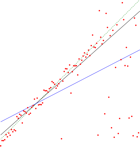
<질문> MSE와 RSE차이?? ### R^2 statistic - RSE는 Y의 단위에서 측정하지만, 절댓값이라 판단하기 어렵다. - R^2는 0에서 1사이 값이기 때문에 Y 단위와 상관이 없기에 fitness를 측정하기에 좋다. R^2은 TSS에 RSS가 가까울 수록 0에 가깝다. TSS 는 회귀를 하기 전 변동성의 합이고, RSS는 regression을 하고 나고서 설명되지 않은 변동성이다. 즉, R^2은 회귀에 의해 설명되지 않은 변동성을 말하기 때문에, 0에 가까울 수록 회귀 모델의 적합도가 떨어진다고 볼 수 있다. - X와 Y사이의 선형 관계를 보여주는 수단이다. - cor(X,Y) 역시 X와 Y사이의 선형 관계를 보여주는데,  where TSS = is the *total sum of squares*, and RSS is defined The *R*2 statistic isa measure of the linear relationship between *X *and *Y *.Recall that *correlation*, defined as  is also a measure of the linear relationshipbetween *X *and *Y *.5 This suggests that we might be able to use *r *=Cor(*X, Y *) instead of *R*2 in order to assess the fit of the linear model. In fact, it canbe shown that in the simple linear regression setting, *R*2 = *r*2. This slightly counterintuitive result is very common in many real life situations. Consider an absurd example to illustrate the point. Running a regression of shark attacks versus ice cream sales for data collected at a given beach community over a period of time would show a positive relationship, similar to that seen between sales and newspaper. Of course no one (yet) has suggested that ice creams should be banned at beaches to reduce shark attacks. In reality, higher temperatures cause more people to visit the beach, which in turn results in more ice cream sales and more shark attacks. A multiple regression of attacks versus ice cream sales and temperature reveals that, as intuition implies, the former predictor is no longer significant after adjusting for temperature. 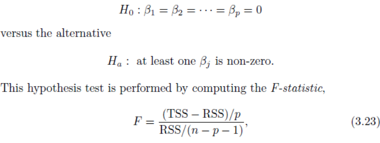### One: Is There a Relationship Between the Response and Predictors?  <질문> It turns out that the answer depends on the values of n and p. When n is large, an F-statistic that is just a little larger than 1 might still provide evidence against H0. In contrast, a larger F-statistic is needed to reject H0 if n is small. 잘설명하면 TSS-RSS 가 1에 가까움,, 1*n --> 저절로 커지게 됨// 통계량이 저절로 작아지게 됨. 잘 못설명하면 0에 가까움 0*n The approach of using an F-statistic to test for any association between the predictors and the response works when p is relatively small, and certainly small compared to n. However, sometimes we have a very large number of variables. If p > n then there are more coefficients βj to estimate than observations from which to estimate them. In this case we cannot even fit the multiple linear regression model using least squares, so the ### Two: Deciding on Important Variables - Forward selection. - Backward selection. - Mixed selection - Backward selection cannot be used if p > n, while forward selection can always be used. Forward selection is a greedy approach, and might include variables early that later become redundant. Mixed selection can remedy this. ### Three: Model Fit - 변수 추가시 R^2 statistics 증가의 문제 : RSE로 해결 It turns out that R2 will always increase when more variables are added to the model, even if those variables are only weakly associated with the response. This is due to the fact that adding another variable to the least squares equations must allow us to fit the training data (though not necessarily the testing data) more accurately. The observant reader may wonder how RSE can increase when newspaper is added to the model given that RSS must decrease. In general RSE is defined as  (3.25) which simplifies to (3.15) for a simple linear regression. Thus, models with more variables can have higher RSE if the decrease in RSS is small relative to the increase in p. ### Four: Predictions However, there are three sorts of uncertainty associated with this prediction. - reducible error --> confidence interval - model bias - irreducible error reducible + irreducible --> prediction interval ​ ## 3.3 Other Considerations in the Regression Model ### 3.3.1 Qualitative Predictors ex  ### 3.3.2 Extensions of the Linear Model **Removing the Additive Assumption- Interaction terms**  The hierarchical principle states that if we include an interaction in a model, we should also include the main effects, even if the p-values associated with principle their coefficients are not significant. In other words, if the interaction between X1 and X2 seems important, then we should include both X1 and X2 in the model even if their coefficient estimates have large p-values. **Non-linear Relationships** mpg = β0 + β1 × horsepower + β2 × horsepower2 +  (3.36) ### 3.3.3 Potential Problems **1. Non-linearity of the Data** Figure 3.9 - Residual plots are a useful graphical tool for identifying non-linearity - If the residual plot indicates that there are non-linear associations in the data, then a simple approach is to use non-linear transformations of the predictors, such as logX, √ X, and X2, **2. Correlation of Error Terms ** - Why might correlations among the error terms occur? Such correlations frequently occur in the context of time series data, which consists of obtime series servations for which measurements are obtained at discrete points in time. - Figure 3.10 - Now there is a clear pattern in the residuals—adjacent residuals tend to take on similar values. **3. Non-constant Variance of Error Terms ** - heteroscedasticity - When faced with this problem, one possible solution is to transform the response Y using a concave function such as log Y or √ Y . **4. Outliers** - Residual plots - observations for which the response yi is unusual given the predictor xi. **5. High Leverage Points ** - Figure 3.13 - high leverage observations tend to have a sizable impact on the estimated regression line. - But in a multiple linear regression with many predictors, it is possible to have an observation that is well within the range of each individual predictor’s values, but that is unusual in terms of the full set of predictors. - quantify an observation’s leverage: For a simple linear regression, statistic hi = 1 n + (xi − ¯x)2 n i=1(xi − ¯x)2 . (3.37) ​ So if a given observation has a leverage statistic that greatly exceeds (p+1)/n, then we may suspect that the corresponding point has high leverage. **6. Collinearity ** Collinearity refers to the situation in which two or more predictor variables are closely related to one another. Figure 3.15  Since collinearity reduces the accuracy of the estimates of the regression coefficients, it causes the standard error for ˆβj to grow. - How to detect collinearity? - correlation matrix -> not always. multi collinearity의 경우는 detection안됨 - variance inflation factor (VIF).  - exceeds 5 or 10 -> serious problem -  - 2 solutions for collinearity - 1. drop one of the problematic variables 2. the average of standardized versions of limit and rating in order to create a new variable that measures credit worthiness. ## 3.5 Comparison of Linear Regression with K-Nearest Neighbors - linear regression - parametric - K-nearest neighbors regression (KNN regression). - non-parametric - 두 개의 성능비교 : the parametric approach will outperform the nonparametric approach if the parametric form that has been selected is close to the true form of f. - true form of f: linear -> linear reg (MSE LOWER)>> KNN - true form of f: NONlinear -> linear reg >> KNN (MSE LOWER) - IN REALITY, however, curse of dimensionality problem occurs. p(predictor 개수)의 개수가 커지면 결국 linear reg >> KNN reg